Learning DAX

---

Data Analysis Expressions (DAX) is the language used to define calculations in the tabular data model. DAX is also the query language used by the client reporting tools to query the tabular data model. In this chapter we will start with basics of DAX (syntax, operators, data types, and evaluation context) and later learn DAX functions.

A DAX query reference contains a number of functions that operate on the column of the table or table itself and evaluates to either a scalar constant or returns a table as well.

DAX syntax

When DAX is used to define calculated columns or measures, the formula always starts with an equal (=) sign. In DAX syntax, the column names of the tables are always referenced within square brackets [ ] and the column names are preceded by the name of the table.

For example, in the previous chapter, we defined the calculated “Name” column in the Employee table using the following formula:

We defined measures in the data model using the following formula:

In these examples, we see that a formula starts with an equal sign and all the columns are referenced as <table-name>[<column-name>].

When DAX is used as a query language to query the tabular data model, the syntax appears as:

DAX as a query language always starts with the EVALUATE keyword followed by an expression, which returns a table.

DAX operators

There are four different types of calculation operators supported by DAX: arithmetic, comparison, text concatenation, and logical.

Arithmetic Operators

Comparison Operators

Text Operators

Logical Operators

DAX operators have the following order of precedence:

1. ^
2. – (Sign operator for negative values)
3. * /
4. ! (NOT Operator)
5. + -
6. &
7. <, >, >=, <=, =, <>

DAX data types

The following data types are supported. When you import data or use a value in a formula, even if the original data source contains a different data type, the data is converted to one of the following data types. Values that result from formulas also use these data types.

In addition, DAX uses a table data type. This data type is used by DAX in many functions, such as aggregations and time intelligence calculations. Some functions require a reference to a table; other functions return a table that can then be used as input to other functions. In some functions that require a table as input, you can specify an expression that evaluates to a table. For some functions, a reference to a base table is required.

Evaluation context

DAX formulas or expressions are always evaluated in one of the following contexts:

• Row context
• Query context
• Filter context

Row context

When a DAX formula is evaluated in row context, the expression is evaluated for each row of the column referenced by the expression. Calculated column expressions are always evaluated in row context.

For example, in our data model we defined the calculated column using the following DAX formula.

This DAX formula is evaluated for each row of the Employee table, and hence is evaluated under the row context of the Employee table.

Query context

When a DAX formula is evaluated in the context of a query, the expression is evaluated by applying the filters defined for that query.

For example:

57.    Dynamically changing query

In this Excel report, as the user clicks on various values of the Country slicer, the DAX query for the pivot table dynamically changes to reflect the filter value selected by the user. In other words, the DAX query is said to be evaluated in the query context.

Filter context

When a DAX formula is evaluated in filter context, the filters defined in the formula override any in the query context or row context. For example, in our data model, we define the following calculated measure:

This formula contains a filter for the fiscal year 2004, so it will always be evaluated under this filter context.

If the measure “FY04 Sales” is used in the Excel report with the slicer setting for fiscal year, the slicer selection does not affect the FY04 Sales measure value because the measure is evaluated in filter context, which overrides the query context.

58.    Filter context in Excel

DAX functions

The DAX language contains a rich set of functions, which makes it a powerful language for analytics and reporting. These functions are categorized into the following:

• Aggregation functions
• Date and time functions
• Filter functions
• Information functions
• Logical functions
• Mathematical and trigonometric functions
• Statistical functions
• Text functions
• Time intelligence functions

Discussing each function in the DAX query reference is beyond the scope of this book; however, we will discuss some commonly used functions from each category.

Aggregation functions

Aggregation functions are used for aggregating the columns. These are primarily useful in defining measures.

The following is a list of aggregation functions available in DAX along with a brief description of each.

Aggregation functions are pretty self-explanatory and simple to use. In the set of functions listed in the previous table, there are variations of the aggregation functions with an “X” suffix, for example, SUMX and AVERAGEX. These functions are used to aggregate an expression over a table or an expression that returns a table. For example, the syntax for the SUMX is:

We can define a calculated measure as follows.

In this formula, the FILTER function first filters the Reseller Sales for France, and later THE SUMX function aggregates the SalesAmount for the sales transactions in France.

The X suffix aggregate function gives us the flexibility to aggregate over a set of rows (or a table) returned from the expression.

Some of the aggregate functions listed in the previous table have an “A” suffix (AVERAGEA, COUNTA). The “A” suffix functions aggregate columns or data with non-numeric data types. All other aggregate functions can aggregate only numeric data types. For example:

When the function does not find any rows to count, the function returns a blank. When there are rows, but none of them meet the specified criteria, then the function returns 0.

The previous DAX formula counts the regions covered by the AdventureWorks Sales Territory, which can used in the following report.

59.    Using an aggregate formula for a non-numeric data type

Date and time functions

In a data warehouse or dimension model, date and time dimensions are conformed dimensions since they are used in all data marts for analyzing measures across dates and times. The Date dimension defined in the data model should have as many columns or attributes as possible (for example, Day, Month, DayOfWeek, MonthOfYear) to give end users the flexibility to identify trends in the data over time.

To support analysis across date and time dimensions, and to extract various attributes from Date columns, we have the following date and time functions.

The functions DAY, MONTH, and YEAR are used to extract the day, month, and year respectively from the date values. For example:

60.    Using date and time functions

Filter functions

Filter functions are another commonly used set of functions, which we have already used in some prior examples. As we slice and dice the measures across the various columns of the table, we filter the data for those values of the columns, which is achieved by using filter functions.

The following table lists the available filter functions.

Although the previous functions are categorized as filter functions, each is unique in the way it filters data. Let us discuss some of the filter functions here.

CALCULATE function

The CALCULATE function is one of the most commonly used functions used to evaluate an expression by applying various filters. Filters defined in the CALCULATE function override the query context in the client tools. For example:

Previously, we defined a calculated measure as FY04 Sales, which uses the CALCULATE function to calculate the sales for the fiscal year 2004:

In the previous DAX formula, the sum of the SalesAmount is evaluated by filtering the Reseller Sales table for the fiscal year 2004. We see that the Fiscal Year column is defined in the Date table, but still it is possible to filter the Reseller Sales table using the fiscal year, due to the relationships defined between the tables. The CALCULATE function automatically uses the active relationship between the tables to filter the expression.

FILTER function

The FILTER function is commonly used to filter a table or expression based on the filter conditions. For example:

In the previous example, to calculate FY04 Sales, we can calculate the same measure using the following DAX formula:

In this formula, we first filter the Reseller Sales table for the fiscal year 2004 and use SUMX to compute the sum of SalesAmount over the filtered Reseller Sales.

RELATED function

The RELATED function is another popular, commonly used function used in calculated columns or measures to perform a lookup to the related table and fetch the column values related by the underlying relationships. The RELATED function uses the underlying table relationships defined during data modeling to perform lookups on the related table.

The RELATED function requires a relationship to exist between the current table and the table with related information. The RELATED function allows users to lookup to the dimension or master tables similar to VLOOKUP for Excel. For example:

In this example, to calculate Total Sales for France, we used the RELATED function:

In this formula, we filter the ResellerSales table using the Country column, which belongs to the SalesTerritory. Hence we use the RELATED function, which uses the relationship defined between the ResellerSales table and SalesTerritory table to filter the ResellerSales table for the country France.

ALL function

The ALL function is used to retrieve all values of a column or table ignoring any filters that might have been applied. This function is useful overriding filters and creating calculations on all the rows in a table. For example:

In our data model, let us say we have a requirement to calculate the contribution of each country to the total sales. In order to create this measure, we define the following calculation:

61.    Using the ALL function

Information functions

Information functions are useful functions to check for the existence of some data value, blank, or error. Most information functions return Boolean values, so they are best used with an IF function.

CONTAINS function

The CONTAINS function returns a Boolean data type (True or False) depending on whether or not the value exists in the specified column. For example:

Consider a scenario where the AdventureWorks management has decided to revise the sales target so that each country should try to meet the sales target of a 20 percent increase, except for the United States. Due to market conditions, management decided to set a target of a10 percent increase for the United States.

To calculate the revised sales target, we use the CONTAINS function as follows:

62. : Using the CONTAINS function

ISBLANK function

The ISBLANK function checks the column value and returns a Boolean value depending on whether the column value is blank.

Blank is a special data type available in the tabular data model that is used to handle nulls. Blank doesn’t mean 0 or a blank text string. Blank is a placeholder used when there is no value. Furthermore, in the tabular data model we do not have nulls, so when the data is imported the nulls are converted to blank values.

The ISBLANK function is useful for checking for blank values within a column. For example:

63.    Using the ISBLANK function in a data model

In this example, we use the ISBLANK function to test whether the current year’s sales are blank, and if they are blank, a blank value is displayed. Further, if the current year’s sales are not blank, we check to see if the previous year’s sales are blank. If they are, we represent a 100-percent increase in sales; otherwise we calculate the percentage growth over the previous year’s sales.

Similarly, we have the ISTEXT, ISNONTEXT, ISERROR, and ISLOGICAL functions which are used to test the value of the column and return Boolean values.

PATH functions

PATH functions are specifically designed to address parent–child dimensions. Unlike the multidimensional model, which automatically detects and creates a parent–child hierarchy, the tabular data model doesn’t support the creation of a parent–child hierarchy out of the box.

In our data model, we have an employee table that has a parent–child relationship in which each row represents an employee who has a manager and the manager in turn is an employee in the same table.

First, we create a calculated column in the Employee table using the PATH function to determine the path of each employee to its parent.

64.    Using the PATH function

As you can see, the column now contains the complete path of EmployeeKey from bottom to top stored as a single string value.

Now, for each level in the parent–child relationship we want to create a column. We use the DAX function PathItem for each calculated column to get the key of a specific level. To get the first level of the path, we use the following function.

To get the second level, we use the following function.

The output of the PathItem function will be EmployeeKey of the manager; however, we need the name of the manager, so we use the LOOKUPVALUE function to look it up as follows.

We define the calculated column for each level of the hierarchy using the previous LOOKUPVALUE function to form a flattened hierarchy as shown in the following figure.

65.    Using PathItem and LOOKUPVALUE to list hierarchy levels

Next, we create an Employees hierarchy by switching to the diagram view:

66.    Creating an Employees hierarchy

Now, we browse the hierarchy in Excel:

67.   Employees hierarchy in Excel

The flaws with each approach for creating a parent–child hierarchy are:

• The number of levels in the parent-child hierarchy should be known in advance so that we can create the calculated column for each level.
• If we have a ragged hierarchy, some levels are blank—hence blank values in the hierarchy in Figure 67. However, we can handle blank values by using the ISBLANK function.

This approach to creating a parent–child hierarchy using Path functions references the following blog by Kasper de Jonge, who is a Microsoft program manager: http://www.powerpivotblog.nl/powerpivot-denali-parent-child-using-dax/

Logical functions

Logical functions are useful in checking, error handling, and performing logical AND/OR operations. The following table lists the logical functions supported by DAX.

Most of the functions listed in this category are self-explanatory and commonly used in other programming languages.

IFERROR is a special function used for error handling in DAX, which we will discuss in more detail. IFERROR is actually a combination of two functions, IF and ISERROR. Since they are commonly used in tandem for error handling, the SSAS product team decided to have a dedicated IFERROR function. For example:

In a previous example, to calculate year-over-year (YoY) percentages, we used the ISBLANK function to handle blank values from the previous year. However, we can also use the IFERROR function to achieve similar results, as shown in the following example.

Mathematical functions

Since DAX is an analytical query language, it has to support mathematical functions useful for analytics and reporting. DAX supports the following mathematical functions.

I believe the functions are pretty self-explanatory and don’t need detailed elaboration. If necessary, we can refer to online documentation for syntax of the functions and put them to use.

Statistical functions

DAX supports the following list of statistical functions. Note that there is some overlap between aggregate and statistical functions (SUMX, COUNT, AVERAGE, etc.).

Some of the statistical functions (such as GENERATE, SUMMARIZE, CROSSJOIN, and TOPN) are useful functions when we use DAX as a query language in client tools. In this section we will discuss RANK functions.

RANKX function

The RANKX function, as the name suggests, is used to rank a column based on an expression or measure. For example:

Consider a scenario where AdventureWorks wishes to rank the products based on their demand and order quantities for the product. To achieve this, we first define a calculated measure, Orders, to capture the order quantity.

Next we use the RANKX function in the Products table to define a calculated column, which ranks the products on the basis of the measure Orders.

68.   Using the RANKX function

Text functions

Text functions are similar to string manipulation functions. These are the text functions available in the DAX query reference:

Most text functions are self-explanatory and pretty straightforward, so we will not discuss them in detail. In fact we have already used FORMAT and CONCATENATE functions in some previous examples.

Time intelligence functions

As discussed previously, date and time are conformed dimensions in the data warehouse as most analysis is performed across the time axis, such as comparing measures like YoY, QoQ, and MoM, and calculating YTD, QTD, and MTD. Time intelligence functions are available to facilitate such calculations.

In order to use time intelligence functions in our data model, we need to have a table marked as a date table and identify one of the columns of that table as a unique identifier, which should be of the date data type.

In our data model, we have a Date table defined which can be marked as a date table, and the column FullDateAlternateKey which is a unique identifier for the table and is of the date data type. In our data model, we mark the Date table by selecting the table and clicking Table > Date > Mark As Date Table as shown in the following figure.

69.    Setting up a table to use time intelligence functions

Next, we click the Date Table Settings option in the same menu, and select the FullDateAlternateKey unique identifier column in the Date field.

70.   Marking a date table

Now that we have marked a date table, we use time intelligence functions to define calculations in our data model.

TotalYTD, TotalQTD, and TotalMTD functions

TotalYTD, TotalQTD, and TotalMTD are functions commonly used in financial analysis to evaluate an expression from the start of the year to the current date, from the start of the quarter to the current date, and from the start of the month to the current date. For example:

In our data model, we define the YTD Sales and QTD Sales measures as follows:

71.    Using the TotalYTD and TotalQTD functions

PREVIOUSYEAR, PREVIOUSQUARTER functions

PREVIOUSDAY, PREVIOUSMONTH, PREVIOUSQUARTER, and PREVIOUSYEAR functions are commonly used functions in financial analysis for comparing the current measure value with the previous day, month, quarter, or year. For example:

In our data model, we can define the measures PreviousYearSales and PreviousQuarterSales, which calculate the sales for previous years and previous quarters using the following DAX formula:

72.    Using PREVIOUSYEAR and PREVIOUSQUARTER Functions

SAMEPERIODLASTYEAR function

The SAMEPERIODLASTYEAR function returns a table that contains a column of dates shifted one year back in time from the dates in the specified date column, in the current context.

The SAMEPERIODLASTYEAR functionality is also possible by using the PARALLELPERIOD function as follows:

For example:

In our data model, we previously defined the calculated measure PreviousSales, which calculates the sales for THE same period last year using the PARALLELPERIOD function as follows:

We can also rewrite this measure using the SAMEPERIODLASTYEAR function to achieve the same result:

Now that we are more familiar with DAX functions, in the next section we will see how we can use some of these functions for reporting.

DAX as a query language

In some of the client reporting tools such as SSRS, we use DAX as a query language to define the dataset to fetch the data from the tabular data model cube. When we use DAX as a query language, we use some of the same functions we discussed earlier, which returns a tabular dataset.

When DAX is used as a query language, we use the following syntax:

DAX as a query language always starts with the EVALUATE keyword followed by an expression, which returns a table. The DEFINE keyword is used to define a calculated measure within the scope of the query.

In order to use DAX as a query language, we use SQL Server Management Studio to connect the tabular Analysis Services cube and click on the New MDX Query window.

The same MDX query window is also used to execute DAX queries against tabular model cubes as shown in Figure 73.

For example, the simplest DAX query would be:

73.    Using DAX as a query language

This query returns SalesTerritory as the output. If the output needs to be sorted by country, we can rewrite the query as:

Applying filters to a DAX query

If we need to evaluate the sales for the fiscal year 2004 for the United States, we use the FILTER function to filter the ResellerSales table for the Country United States and FiscalYear 2004. The resulting DAX query is:

Adding columns to query output in a DAX query

Consider a report where we need all the products in the AdventureWorks catalog along with their max quantities ordered to date. We can use the ADDCOLUMNS function to add a calculated column that computes the max order quantity and adds it to the product table. The resulting DAX query is:

Aggregating and grouping in a DAX query

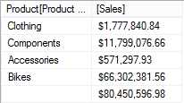
Consider a report where we need the aggregated Sales value for each Product Category. This can be easily achieved in a DAX query by using the SUMMARIZE function as follows:

74.   Using a DAX query to aggregate values

If we want to compute total sales as well, we can use the SUMMARIZE function along with ROLLUP in the DAX query:

75.    Using a DAX query to aggregate values

Using CROSSJOIN in a DAX query

Consider a report where we need to compute the sales for each country, for each fiscal year. We can use the CROSSJOIN function to achieve this as shown in the following DAX query:

76.    Using CROSSJOIN in a DAX query

Using TOPN in a DAX query

Consider a report where we need to identify the top three products that are in demand. To achieve this, we will use the TOPN function and the Demand Rank calculated column defined previously, which calculates the rank for each product based on the total order quantities sold to date.

77.  Using the TOPN function in a DAX query

Define measures in a DAX query

In the previous example where we designed a DAX query to calculate the max quantities sold for each product to date, we can rewrite the query by defining the measure as shown in the following sample.

Defining query-scoped measures simplifies the query to a large extent. For instance, in the previous query we first define a calculated measure to compute the max order quantity sold for all products. When this measure is used within the ADDCOLUMNS function, the measure is evaluated in row context for each row of the product table, which gives the max order quantity for each product.

Using the GENERATE function in a DAX query

In the previous example, we calculated the top three products in demand based on the total order quantities sold using TOPN. Now, let us say we need to calculate the top three products in demand for each country to identify the most popular products in each country.

To do this, we need to iterate the same TOPN calculation for each country. This is possible using the GENERATE function in DAX as follows.

In this DAX query, we repeat the TOPN calculation which calculates the top three products based on the max order quantities sold for each country using the GENERATE function. The resulting output of the query is shown in the following figure:

78.   Using the GENERATE function in a DAX query

These examples should give us enough exposure to get started with DAX. Like with any other query language, we can achieve expertise in DAX with more practice.

Summary

In this chapter, we learned how to define calculated columns and measures using the DAX language. In the next chapter, we will discuss how to prepare our data model for deployment and deploying the data model for reporting and analytics.