Developing a Data Model with a SSAS Tabular Instance

---

In this chapter, we will start with designing and developing a data model with the SSAS tabular instance using SQL Server Data Tools (SSDT, formerly called BI Development Studio).

As discussed in the previous chapter, unlike the multidimensional model approach, the tabular data model doesn’t necessarily require data to be organized in dimensions or facts in the data warehouse. This makes tabular data modeling a preferred approach for relatively small data warehouse designs wherein the data might be available in disparate data sources, which can be directly loaded into the SSAS tabular data model for analytics. However, designing a data warehouse in a star or snowflake schema remains the recommended approach, since it stores the consolidated historical data, which decouples the data from the original (and potentially changing) data.

In this chapter we will use the AdventureWorksDW2012 database as our data source for the tabular data model. The AdventureWorksDW2012 database is a sample data warehouse database available from www.codeplex.com. The sample databases can be downloaded from this link.

Scenario

AdventureWorks is a virtual company that sells bikes, bike accessories, bike components, and clothing. The company sells its products through an online portal as well as through resellers. Each sales transaction via the Internet or a reseller is captured in an OLTP database (AdventureWorks2012), while AdventureWorksDW2012 is the corresponding data warehouse for this OLTP database where the data is organized in a star schema into dimension tables and fact tables.

The business analyst in the organization needs to analyze the reseller sales by geography; by product size, color, and weight; by its employees; and by date dimensions dynamically. For the given requirements, we have the following star schema designed in the AdventureWorksDW2012 data warehouse database.

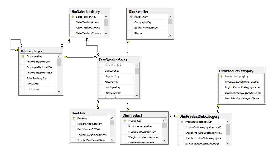
12.   AdventureWorksDW2012 Schema

The requirement is to design a tabular data model for the reseller sales data mart so that business analysts can use Power View or Excel to dynamically sort the sales data to fetch reports for analytics.

Let’s start by developing our Analysis Services tabular project in SSDT to understand the approach for data modeling.

Getting started with an Analysis Services tabular project

Similar to the multidimensional cube, SQL Server Data Tools (SSDT) is used to design and develop the SSAS tabular model cube. During the installation of SSAS, there is an option to select multidimensional mode or tabular mode when we reach the server configuration page for Analysis Services. A given instance of SQL Server can have Analysis Services in either multidimensional mode or tabular mode. However, if we need to install both modes of SSAS on the server, we will need to install two instances of SQL Server (run the setup again to install another instance).

On my development workstation, I installed a default instance of SQL Server that contains Database Engine, SSAS in multidimensional mode, SSRS, and shared components, and I installed a named instance of SQL Server (TABULAR) to install an SSAS tabular model.

After installation, when we start SSDT and click New Project, we will see the following templates available for business intelligence:

13.   Business intelligence project templates

The Analysis Services Tabular Project is the new template available in SSDT.

In the New Project window, we name our project AdventureWorks Reseller Sales and click OK to create the project. The following window appears.

14.   Tabular model designer

The Tabular model designer requires us to provide the SSAS tabular instance name, which will be used as a workspace server during the development of the project. During the development phase, when we process the data into the data model, it will actually be stored in a temporary database created in a workspace SSAS instance.

It is important to understand that a workspace server is not the instance where the tabular model cube will be deployed; the deployment instance will be separate and needs to be specified separately, which we will discuss further during deployment.

Whenever you create or open a tabular project, a workspace database is saved in the server’s OLAP\Data directory. Over time, this folder may be bloated with temporary databases. From time to time you will need to get rid of the stuff in there you don’t need anymore. To do that, you need file system access. Therefore, it is best if you pick a workspace database server that you can clean up. This is not required, but your server administrator will thank you.

In the first screen of the Tabular model designer, we provide our SSAS tabular instance name and click Test Connection to ensure we are able to connect to the workspace server. If the test connection fails, either the server name provided is incorrect, the server might not be reachable due to a firewall or other reasons, or the Windows credentials with which you logged in do not have permissions on the SSAS instance.

In this screen, we also have a Compatibility Level menu where we have two available values (at the time of writing this book):

• SQL Server 2012 RTM (1100)
• SQL Server 2012 SP1 (1103)

Each tabular model database is associated with a version of SQL Server it is compatible with and can be deployed to. If we are developing a tabular data model that will be deployed to an SQL Server 2012 SP1 instance, we should select the compatibility level as SQL Server 2012 SP1 (1103), and vice versa.

After specifying the workspace server and compatibility level details, click OK. The solution is created and an empty file called Model.bim is opened, as shown in the following figure.

15.    New project

Import data to the tabular model

As discussed previously, the first step in designing a data model is to identify the data sources for the data. For the given requirements, we have all the required data available in the AdventureWorksDW2012 file.

In order to import the data from data sources, in SSDT, click the Import from Data Sources button, which is the first option in the toolbar at the top left corner as shown in the following figure.

16.    Import from Data Sources button

When we click the Import from Data Sources button, the Table Import Wizard pops up and shows all the supported data sources.

17.   Supported data sources for the tabular model

As shown in the previous figure, the tabular model project supports a wide range of data sources, including relational databases, SQL Azure, multidimensional cubes, flat files, and data feeds.

Select Microsoft SQL Server and click Next. In the next screen we provide the connection string for SQL Server by providing the server name and selecting AdventureWorksDWDenali (which is our AdventureWorksDW2012 database) in the Database name drop-down. We provide a Friendly connection name as AdventureworksDW to easily identify the data source.

Note: For all my demos and labs I have used the AdventureWorksDWDenali database, which was available as a sample database in the CTP version of SQL 2012. When you download the latest AdventureWorksDW2012 from the CodePlex site, the database name will be AdventureWorksDW2012, and the data might be different from the demos and labs displayed in this book.

Before moving to the next screen, it is important to click Test Connection to ensure the connection to the database is successful and does not result in any errors.

18.   Setting up the database connection

Next, we need to provide Windows credentials which will be stored in the tabular model cube, and will be used to connect to the AdventureWorksDW2012 database to move data into the tables of the data model.

If the SSAS Service Account has permissions to read data from the data source, we can select the Service Account option, which does not require us to provide the credentials explicitly. This might be the preferred approach if the service account is a domain account and has permissions for the data source, which might be on a remote server.

19.   Setting up Analysis Services credentials

The next screen allows us to import data directly by selecting the table or by writing a SQL query, which might be useful if we want to join multiple tables and import the data into a single table. Click Select from the list of the table to advance to the next step.

In this step, we select the individual tables that we would like to import and provide a user-friendly name, which will be the name for the imported table in the data model.

20.   Selecting tables to import

For our data model, we select the following tables and provide the following names.

For the DimSalesTerritory, we filter out the SalesTerritoryAlternateKey column by clicking the DimSalesTerritory table and selecting the Preview and Filter option as shown in the following figure.

21.   Filtering a column from the DimSalesTerritory table

In the same window, we can set row filters by clicking the drop-down next to each column header and selecting the boxes that need to be filtered.

In order to improve the processing time and save storage space, it is always recommended to filter out unrequired columns and rows.

In our scenario as well, we have a number of such columns that can be filtered out in each table, but to keep things simple, we will only filter out a column from DimSalesTerritory as shown in the following figure.

22.   Filtered DimSalesTerritory source

Once we have all the required tables selected and necessary filters applied, we can click Finish to import the data into the tables in the data model. For a SQL Server data source, we also import relationships along with the data, which are visible in the last step, data preparation. For other data sources, we need to create relationships manually in the data model.

23.   Importing data

Next we need to import the tables DimProduct, DimProductSubCategory, and DimProductCategory, but we do not need them to be imported as three separate tables. Instead, we would like to denormalize the three tables into a single table called columns.

To do this, we need to start the Table Import Wizard again and import the table by writing a SQL query that joins the three tables and imports the required columns.

Since we already have the connection to AdventureWorksDW2012 created, we can click the Existing Connections option on the toolbar to launch the Table Import Wizard as shown in the following figure.

24.    Existing Connections button

25.    List of existing connections

Select AdventureWorksDW, and then click Open. The next window will give you options for how to import the data. Select the Write a query that will specify the data to import option.

26.    Data import options

Next, we type the following TSQL query, which imports the data from multiple tables (DimProduct, DimProductCategory, and DimProductSubCategory).

27.    Typing a query to import data from multiple tables

Name the table Product and click Finish to import the data.

Note: For development purposes, while designing the Tabular Model in SSDT, it is recommended to import only a subset of the original database since all the data processing resides in a temporary workspace database on the workspace server instance.

We have now imported the following five tables from the data source into the tabular model:

28.    Imported tables

Modifying or deleting an imported table

If you are not happy with the table or columns that you imported from the table, you can delete a table or modify its columns. First, click the tab of the table you want to change at the bottom of the window. The following figure shows the Reseller Sales table being selected. Next, click the Table option in the menu. As the name suggests, the Delete Table option allows you to delete the table, while selecting Table Properties allows you to modify the table or the TSQL query used to import the table.

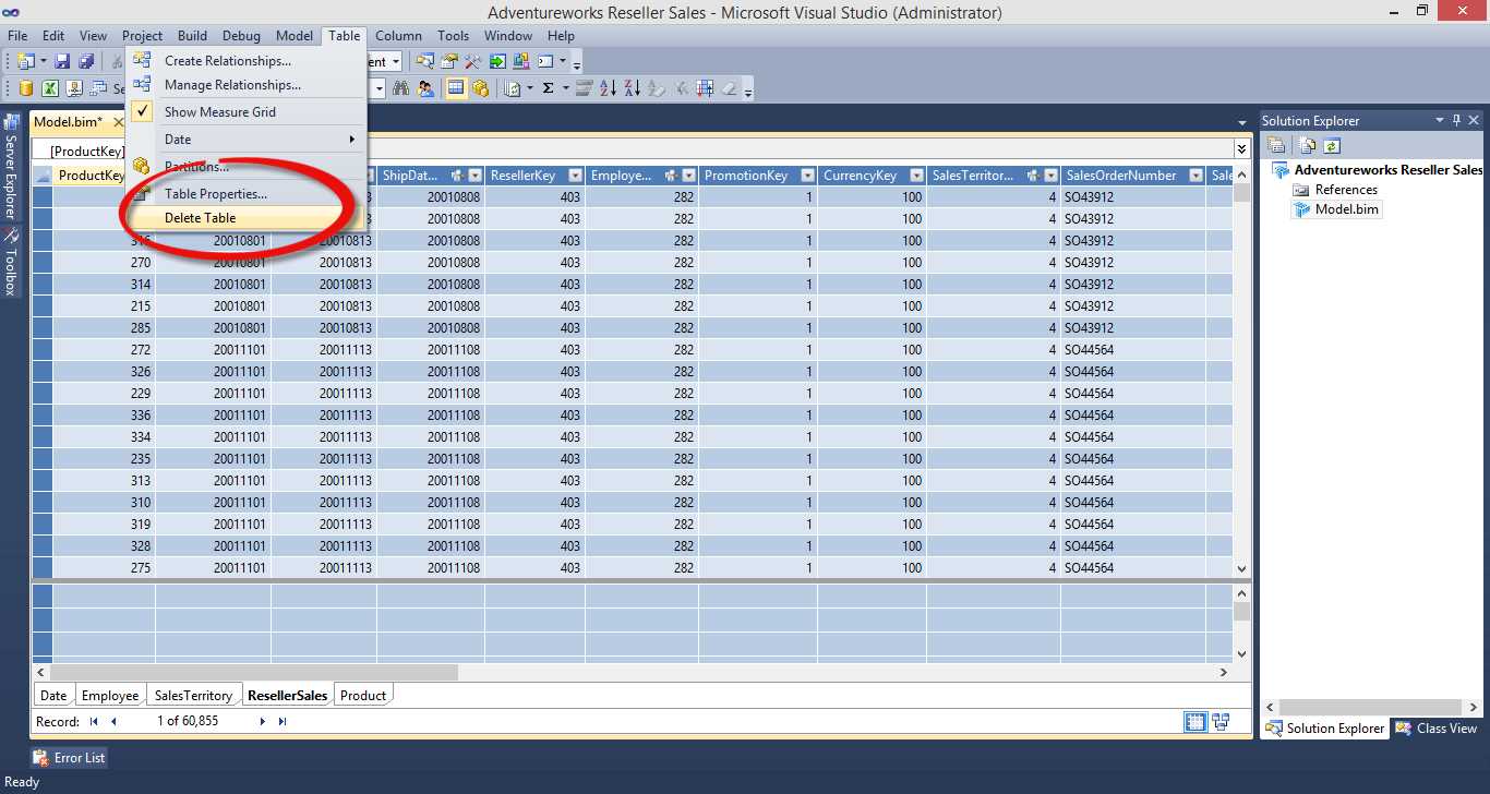
29.    Deleting a table

Modifying or deleting a column in the table

We can either rename, filter, or delete a column after it is imported by selecting the column and right-clicking on it as shown in the following figure.

30.    Modifying a column

In our data model, we imported all tables but we couldn’t provide the column name (we can provide a column name in a SQL query by using a column alias, which we missed in the previous query). After the data is imported into tables, it is important to rename the columns to user-friendly names since the data model will be exposed to end users as is.

We will rename the following columns with new, user-friendly names:

Similarly, using the Table Import Wizard, we can import the data from various other data sources.

The following is a list of data sources supported by the tabular data model:

In this section we imported the data from data sources into the data model. In the following section we will design the hierarchies, relationships, and KPIs to enhance the model for reporting.

Defining relationships

Once all the required data is imported in the data model and after applying the relevant filters, we should next define relationships between the tables.

Unlike RDBMS, which uses relationships to define constraints (either primary key or foreign key), we will define relationships in the tabular data model to use them in DAX formulas while defining calculated columns and measures. There are DAX formulas such as USERELATIONSHIP, RELATED, and RELATEDTABLE used in defining calculations that are purely dependent on relationships.

While importing the data from the SQL server data source, when we select multiple tables from the SQL database, the Table Import Wizard automatically detects the relationships defined in the database and imports them along with data in the data preparation phase. For other data sources, we need to manually create relationships after data has been imported.

In our case, since we imported the Product table by running the Table Import Wizard again, the relationship for the Product table is not automatically imported. We need to manually create the relationship.

There are two ways to create relationships.

In the first way, we click on the Reseller Sales table which has the foreign key ProductKey column, click the Table tab, and select Create Relationships as shown in the following figure.

31.   Create Relationships menu item

This opens the Create Relationship window. We can provide the Related Lookup Table and Related Lookup Column as shown in the following figure.

32.    Create Relationship window

We can also define relationships using the diagram view. We can switch to diagram view by clicking the Diagram option at the lower-right corner of the project, as shown in the following figure.

33.    Diagram view option

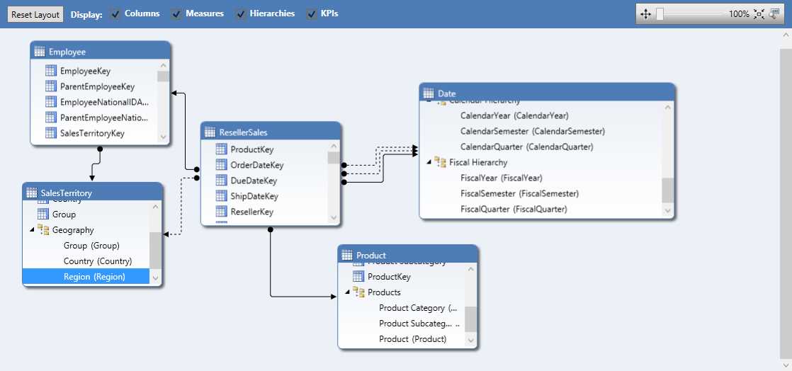
In the diagram view, we can drag the ProductKey column from the ResellerSales table to the ProductKey column in the Product table and the relationship will be created as shown in the following figure.

34.    Using the diagram view to create relationships

The diagram view is useful for seeing all the tables and their relationships, especially when we are dealing with large, complex data marts.

In diagram view, the solid lines connecting tables are called active relationships, and the dotted lines connecting tables are called inactive relationships.

We see inactive relationships when a table is related to another table with multiple relationships. For example, in the previous diagram, the Date table is a role-playing dimension, and hence it is related to the Reseller Sales table with multiple relationships (OrderDateKey, DueDateKey, and CloseDateKey). In this case, only one relationship can be considered active, which will be used by the RELATED and RELATEDTABLE DAX functions, while the other two relationships are considered inactive and can be used with the UseRelationship DAX function.

We can switch an inactive relationship to active by right-clicking on the dotted inactive relationship and selecting Mark as Active, as shown in the following figure.

35.    Changing a relationship to active

Now that we have defined the relationships, we will learn how to define hierarchies.

Defining hierarchies

Hierarchies are very useful for analytics as users navigate from high-level aggregated data to detailed data. Hence, it is important that the cube or data model supports the creation of hierarchies to allow users to drill down or roll up the data. Most dimension tables contain hierarchical data.

For example, the time dimension can have the hierarchy: Year > Semester > Quarter > Monthly > Weekly > Day. The Geography dimension can have the hierarchy Country > State > City.

The characteristics of a hierarchy are:

• It contains multiple levels starting from the parent level to the child level.
• Each parent can have multiple children, but a child can belong to only one parent.

In our data model, we can have following hierarchies:

In order to create hierarchies, we need to switch to the diagram view. At the header of each table in the diagram view, we see an option to create a hierarchy.

36.    Create Hierarchy button in diagram view

When we click Create Hierarchy, it will create a new hierarchy object, which we name Calendar Hierarchy, as shown in the following figure.

37.    Creating a new hierarchy

Next, we drag the CalendarYear column from the table to the Calendar Hierarchy, followed by CalendarSemester and CalendarQuarter to form the Calendar Hierarchy as shown in the following figure.

38.    Creating the Calendar Hierarchy

Similarly, we create Fiscal, Products, and Geography hierarchies.

39.    Fiscal, Geography, and Product hierarchies

Defining calculated columns

Calculated columns are nothing but derived columns defined using DAX formulas. Calculated columns are evaluated in row context, or in other words, for each row of the table.

In our data model, we have the Employee table in which FirstName, MiddleName, and LastName for each employee is captured in a separate column. However, for reporting and analytics, it would make sense to represent employees with their full name (FirstName + MiddleName + LastName). To do this, we define a calculated column called Name in the Employee Table to concatenate FirstName, MiddleName, and LastName of each employee.

To add a calculated column, we go to the Employee table and scroll right until we reach the last column. In the column after the last column we can start typing our DAX formula to define a calculated column.

40.    Adding a calculated column

By default, the column will be named CalculatedColumn1, which we need to rename as Name by right-clicking on the column as discussed previously.

In our data model, CalendarQuarter and FiscalQuarter are represented by numeric values 1, 2, 3, and 4; however, from a reporting perspective, quarters are represented as Q1, Q2, Q3, and Q4. Hence we define a calculated column using the following DAX formula:

Defining calculated measures

Calculated measures are measures of interest that are aggregated across various dimensions and levels of the dimension hierarchy.

In our data model, the ResellerSales table originates from a fact table that consists of the key columns used to look up the dimensions table and measure columns, which need to be aggregated. One of the key measures of interest in the Reseller Sales table is Sales Amount, which needs to be summed up across various dimensions. For this reason, we need to define a calculated measure called Sales to calculate the summation of Sales Amount.

Calculated measures need to be defined in the measure grid, which is visible in the section below the table tabs as shown in Figure 41. We define the calculated measure Sales using the following DAX formula.

Note: Do not worry about the DAX syntax at this point. We will cover DAX in detail in the following chapter.

41.    Defining a calculated measure in the measure grid

Next, we define the calculated measures Cost, Profit, and Margin using the following DAX formulas.

Formatting the calculated measures to currency and percentage formats as displayed in the following figure is explained later in the book.

42.   Measures with unit formatting

We will define more calculated measures as we learn DAX in the following chapter. In the next section we learn about defining KPIs.

Defining KPIs

Key performance indicators (KPIs) are the graphical and intuitive representation of the relationship between a measure and a goal.

As shown in the following figure, KPIs are status or trend indicators that can be used to highlight deviation of a measure from a goal.

43.   KPIs

In our data model, we have defined the calculated measure Margin, which calculates the percentage profit over cost. Now, the organization wants to set up a KPI such that if the margin is more than 0.8 percent of the cost it is considered good, if the margin is between 0.4 and 0.8 percent, the profit is moderately good or average, and if the margin is less than 0.2 percent, it is considered poor.

To analyze the Margin, we define a KPI by selecting the cell where we have Margin defined, right-click it, and select Create KPI as shown in the following figure.

44.    Create KPI option

In the KPI window, the Margin measure is already selected, and we can set the goal or target as an absolute value by clicking the Absolute value option and setting the value of the goal to “1” as shown in the following figure. We then select the status thresholds as 0.2 for the lower band and 0.8 for the upper band, and select the KPI icon style as the red, yellow, and green circular indicators.

45.    Setting up a KPI

Once we click OK, the KPI is created in the data model for the Margin measure. In order to verify the KPI we can browse the data model in Excel by clicking on the Excel icon in the top left toolbar of the project:

46.    Analyze in Excel option

This opens an authentication window as shown in the following figure. We need to log in and open Excel using the Current Windows User option and click OK. The authentication and security is covered later in this book.

47.    User options for analyzing the data model in Excel

Excel will open with a pivot table and a data connection to the model. In the PivotTable Fields window, we can drag the Geography hierarchy to the Rows area, and drag Sales, Cost, KPI Value, Margin, and KPI Status to the Values area as shown in the following figure. The resulting Excel report follows:

48.    Data model analyzed in Excel

Filtering the data model

There are two ways to filter the row data:

• Filter the data while importing from a data source
• Filter the data after importing from a table

The first option is the preferred method; filtering the data while importing from a data source will help reduce the processing time and storage requirements. In the Importing data section, we discussed the various filter options. In this section, we will discuss filtering the data after it’s loaded in the data model.

After the data is loaded, we can have the following filters depending on the data type of the column:

• Number filters
• Text filters
• Date filters

To filter the rows based on any of the columns, we need to click the drop-down arrow next to the column to see the filter options.

49.    Number filter options

50.    Date filter options

51.   Text filter options

As shown in the previous figures, when we click the numeric column DateKey we see number filters, when we click the date column FullDateAlternateKey we see date filters, and when we click on the text column EnglishDayNameOfWeek we see text filters.

If we define a filter for any of the columns of the table, we see the following icon next to the column header:

52.    Filtered column header

Filtering the data in the data model might be a good option if we want to temporarily filter the data for some requirement and remove it later.

Sorting the data model

As shown in the previous figure, clicking the drop-down on a column header opens an option to sort the column in either ascending or descending order.

Depending on the data type of the column, the following options are available for sorting.

Besides these sorting options, we have additional options to sort a column based on the values of another column. These are very useful and are in fact required in some scenarios.

In our data model, we have a Month column in the date table. The Month column is of text data type, and if we try to sort the month column by its own data values we will see the following report:

53.   Sorted Month column

In this report, the data is sorted by the Month values in ascending order with April at the top and September at the bottom, but this is not what we want. We would like the Month column to be sorted based on the order of months throughout the year instead of alphabetically. To do this, we will need to sort based on the MonthNumberOfYear column.

To do this, we use the Sort by Column option as shown in the following figure:

54.    Sort by Column button

55.    Sort by Column options

We select the Month column, click Sort by Column, and select MonthNumberOfYear as the By Column. This will sort the Month column by MonthNumberOfYear and will give us the report in the expected order.

56.    Month column sorted by MonthNumberOfYear column

Summary

In this chapter, we learned about developing a data model with SSAS tabular model using SSDT. In the next chapter, we will focus on the DAX language, which is used to define calculated columns and measures as well as query language for the tabular model.