Queries with DocumentDB

---

Introduction

In the previous chapters, I’ve explained the benefits of using Cosmos DB with the DocumentDB API and we’ve learned about some of its most prominent features.

We described how DocumentDB is designed from the ground up to scale out and work with schema-free hierarchical JSON documents instead of traditional database tables.

We also explored how to get up and running with Cosmos DB (DocumentDB API) using the Azure Portal by creating a database and a collection. We also learned how to import data using the Data Migration Tool.

With this wrapped up, we are in a position to fully start using DocumentDB, putting some data in it and executing queries.

In this chapter we’ll explore how to query DocumentDB using a very familiar SQL-like grammar and syntax for retrieving documents, with roots in JSON and JavaScript semantics.

The Microsoft Azure Cosmos DB team has made a great decision to use a SQL flavored syntax for querying documents within DocumentDB, as it is expressive, easy-to-use, and standard (most developers know it), rather than coming up with a new language or way of querying documents.

What is important to understand is that SQL is actually a relational database querying language. However, Microsoft has adapted it to the NoSQL world, so it is capable of querying JSON documents and establishing relations among them, just like it does with a relational database.

The language still reads as traditional SQL, but the semantics are all based on JSON and it works with JavaScript, but not T-SQL datatypes. Also, expressions are evaluated as JavaScript expressions rather than T-SQL ones.

It is also important to understand that the results returned by running DocumentDB queries using the SQL flavored syntax will be schema-free JSON objects, which could have nested properties or not. We will not be dealing with results organized into rows and columns using a tabular format. Nested properties are accessed using dotted notation, which allows you to descend into any subsection of a document.

The beauty of the SQL flavored syntax in Cosmos DB using the DocumentDB API is that it also allows you to iterate through nested arrays among documents and project the results as a custom JSON document to fit your needs or simply return the results as-is.

The usage of common operators is also allowed, such as arithmetic operators (+, -, *, /, %), bitwise operators (|, &, ^, >>, >>>), logical operators (AND, OR), comparison operators (=, !=, >, >=, <, <=, <>), and the string operator for concatenation (||).

Furthermore, the usage of clauses such as SELECT, FROM, WHERE, JOIN, IN, BETWEEN, and ORDER BY are permitted.

There are many built-in functions for:

• Math: ABS, CEILING, EXP, FLOOR, LOG, LOG10, POWER, ROUND, SIGN, SQRT, SQUARE, TRUNC, ACOS, ASIN, ATAN, ATN2, COS, COT, DEGREES, PI, RADIANS, SIN, and TAN.
• Type checking: IS_ARRAY, IS_BOOL, IS_NULL, IS_NUMBER, IS_OBJECT, IS_STRING, IS_DEFINED, and IS_PRIMITIVE.
• String: CONCAT, CONTAINS, ENDSWITH, INDEX_OF, LEFT, LENGTH, LOWER, LTRIM, REPLACE, REPLICATE, REVERSE, RIGHT, RTRIM, STARTSWITH, SUBSTRING, and UPPER.
• Array manipulation: ARRAY_CONCAT, ARRAY_CONTAINS, ARRAY_LENGTH, and ARRAY_SLICE.

Although we won’t explore each and every one of these built-in functions, it’s useful to know that the DocumentDB SQL flavored syntax supports all these options, which makes it convenient for handling documents with various data types. The functions will also be useful when projecting custom JSON results.

By the end of this chapter you should have a good understanding of how to write and execute queries using DocumentDB to retrieve documents and project custom results. The examples should be both intuitive and easy to follow and implement.

I encourage you to explore the online documentation, which contains a wealth of information about DocumentDB’s query language.

Now, let’s get started and explore how we can query DocumentDB using its very own SQL flavored syntax. Let the fun begin!

Our first query

The Azure Portal has a Query Explorer that allows us to run queries against DocumentDB collections.

We’ll be actively working with the Query Explorer to showcase the various possibilities of querying DocumentDB.

To get started, within the Data Explorer (Preview) blade, select the Items collection and click the ellipsis (…) button. A small menu will appear with a few options. Then click the New SQL Query option. This will open a query tab as shown in the following figure.

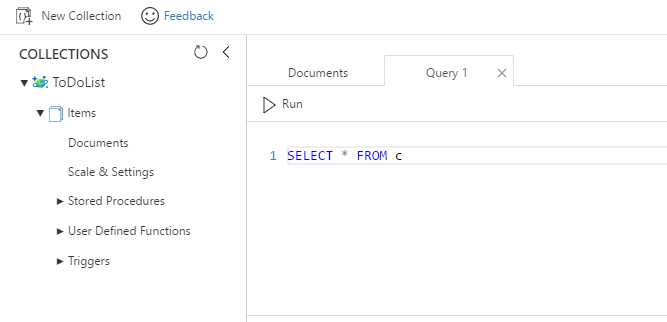
Figure 3-a: A Query Explorer Tab

As soon as the Query Explorer tab is opened, a default query is presented. This query is a simple SELECT * from the active collection.

Code Listing 3-a: The Default DocumentDB Query

To execute the query, you must click the Run button at the top of the Query tab. Notice that in the Query tab, queries are not terminated using a semicolon (;).

Based on the collection we previously created containing information about Cristiano Ronaldo, this is what the result looks like after running the query.

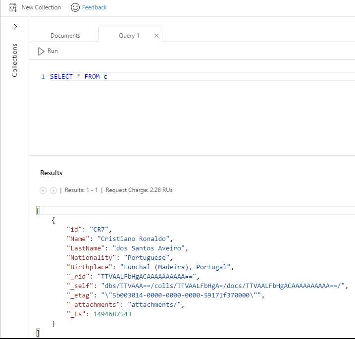
Figure 3-b: The Query Result

Notice that the resulting document contains additional properties that were not originally visible when the document was added to the collection.

These properties are the document’s resource ID (_rid); time stamp (_ts), which represents a raw integer value for when the document was last inserted or updated; self-link (_self), which drills down on _rid from the database to the collection and to this specific document; _etag, used for concurrency; and the _attachments link (in case there are any).

Although this is a very simple query, there are some important differences from the world of relational databases. In a relational database, * means all the columns. In DocumentDB, * means return the document results as they are stored.

Unlike with relational databases, using * doesn’t have any negative impact on performance. If you specifically indicate the name of the properties you want to include in your results, then you are projecting a new shape for each document that will be returned within those results, therefore providing a consistent schema for those returned documents. In DocumentDB, this is known as projection.

The FROM clause is used to indicate the collection the query will be executed against. It is not mandatory to use it. However, if it is not used, then you will not retrieve documents stored within a collection, but instead be executing queries with expressions that return scalar values. We’ll explore that shortly.

At the top of the Results area, DocumentDB provides some valuable information about the RUs involved when executing this query.

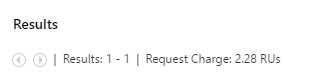
Figure 3-c: Query Execution RU Details

This wraps up our first query. Now that we know how to create a new query, let’s move on to more advanced examples and interesting things we can do. Scalar queries are up next.

Basic scalar queries

Scalar queries are queries that simply evaluate expressions and do not return any document results from a collection. These queries are a great way to learn the basics of DocumentDB querying and explore what is possible. They are also very useful when building custom projections.

Let’s have a look at some basic scalar expression queries.

Code Listing 3-b: Basic Scalar Queries

Let’s now execute each one of these queries separately with our opened Query tab.

If you copy and paste these three queries directly into the Query tab, you won’t be able to execute them all at the same time.

In order to execute these queries one at a time, copy, paste, and then run each one separately.

Let’s start off by running the first one. This query returns the following result.

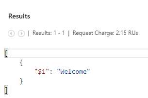
Figure 3-d: Scalar Query 1 Execution Result

Notice how DocumentDB created a JSON document using the expression passed as its result. However, look at what happens when we execute the second query.

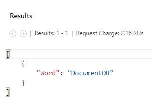
Figure 3-e: Scalar Query 2 Execution Result

In this case, the name of the property is Word instead of $1. This is because in the second query we used the AS clause to indicate how we want to represent the result.

In the first query, because the AS clause was not used, DocumentDB automatically assigned the name $1 to the resultant property of the query.

When we execute the third query, we get the following.

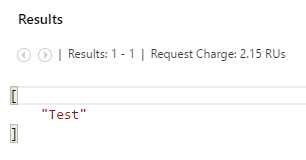
Figure 3-f: Scalar Query 3 Execution Result

In this query, because we are using the keyword VALUE, we are telling DocumentDB to simply return the value of the expression without a property name.

Now let’s consider these other examples that show a very cool feature of DocumentDB’s SQL flavored querying syntax: the ability to include JSON expressions.

Code Listing 3-c: Scalar Queries with JSON Syntax

If we copy and paste the first query and click Run, we’ll get the following result.

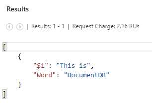
Figure 3-g: Another Scalar Query Execution Result

As you can see, the result is pretty much what we were expecting, given that the second string “DocumentDB” was projected into the property Word using the AS clause, whereas for the first string “This is”, DocumentDB created an automatic property called $1.

Now, copy, paste, and execute the second query. Running the query provides the following result.

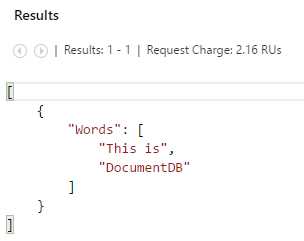
Figure 3-h: JSON Syntax Scalar Query Execution Result

Notice in this query that DocumentDB is returning the result containing the two words as an array, just like it was represented as an expression using JSON syntax.

Being able to include JSON syntax in the SQL expression itself is a very handy and powerful feature, which can be quite valuable when creating custom projected results.

Let’s explore other types of scalar expression queries we could use and run with DocumentDB.

Advanced scalar queries with JSON syntax

So far we’ve seen some simple and interesting scalar queries we can write using DocumentDB, but we’ve just scratched the surface of what kind of scalar queries are possible. Let’s have a look at the following examples.

Code Listing 3-d: More Scalar Queries with JSON Syntax

If we copy, paste, and then run the first example on the Query tab, we get the following result.

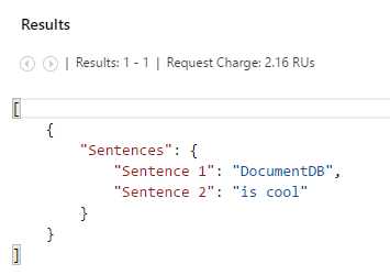
Figure 3-i: JSON Syntax Scalar Query Execution Result

If we copy, paste, and run the second example, we get the following result instead.

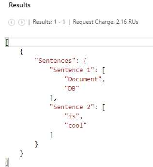
Figure 3-j: JSON Syntax Scalar Query Execution Result

Notice that main difference between these scalar queries is that in the second example Sentence 1 and Sentence 2 are actually array properties, whereas in the first example they are simply string properties.

You can let your imagination go wild. Basically, any kind of projection can be shaped. That’s the expressiveness and beauty of what can be achieved with JSON syntax inside a scalar query.

Scalar queries using operators

Scalar queries are flexible and very versatile. One of their great features is that they can be used with operators. Let’s have a look at what is possible.

Code Listing 3-e: Scalar Query Using Operators

This scalar query includes a few interesting things. It includes both mathematical and logical operations. It also includes a ternary and coalesce expression, as well as string concatenation.

When running this example, the following result is projected.

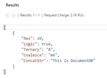
Figure 3-k: Result of the Scalar Query Using Operators

We can combine all sorts of operations together as long as they make sense in order to project custom fields. The ternary and coalesce operators can be used to build conditional expressions similar to other popular programming languages.

The ternary (?) operator can be very handy when constructing new JSON properties on the fly. On the other hand, the coalesce (??) operator can be used to efficiently check for the presence of a property defined in a document. This is useful when querying against semi-structured data or data of mixed types.

We can use parentheses to determine the correct order in which we want expressions to be evaluated, just like we would do with JavaScript expressions. The same expression evaluation rules as in JavaScript apply here as well.

Furthermore, coalesce expressions can be chained to one another, and even string concatenations are possible. The possibilities are endless, limited only by the operators available and your imagination.

More information about DocumentDB query operators can be found here. Up next are scalar queries using built-in functions. Let’s have a look.

Scalar queries using built-in functions

Beyond using operators, we can also write scalar queries using many of the useful built-in functions provided by DocumentDB. Let’s explore some examples.

Code Listing 3-f: Scalar Query Using Built-In Math Functions

If we copy and paste this text and execute this query, we get the following result.

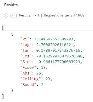
Figure 3-l: Result of the Scalar Query Using Built-In Functions

DocumentDB’s built-in math functions work just as great and in the same way as math functions from other platforms and programming languages, using the same intuitive and well-known names. Details about each math function can be found here.

Let’s now look at running a query using built-in functions to perform type checking on specific data types. Type checking functions are indispensable when you have one or more properties with varying data types.

Code Listing 3-g: Scalar Query Using Built-In Type Checking Functions

If we execute this query, we get this result.

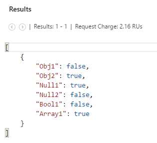
Figure 3-m: Result of the Scalar Query Using Type Checking Functions

Type checking functions are really useful because you may know that a property exists in some documents within a collection, but you may not know what data type that property actually is. Even properties with the same name throughout different documents might have different data types. Type checking is a very useful way of ensuring you use the right data types for the results you need to project.

Now that we’ve quickly explored type checking functions, let’s move our attention to built-in string manipulation functions. These include features such as string extraction, parsing, case conversion, concatenation, and search. Let’s explore an example.

Code Listing 3-h: Scalar Query Using Built-In String Manipulation Functions

String manipulation functions are self-descriptive and have been designed to work in DocumentDB in the same way they have been designed to work in other programming languages.

If we execute this query, we get this result.

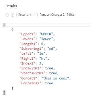
Figure 3-n: Result of the Scalar Query Using String Manipulation Functions

The results are also very much self-explanatory and easy to understand just by looking at them. String manipulation functions provide a great way to project custom query results.

More details about each individual string manipulation function can be found here. Have a look to understand what each one does.

Now that we’ve explored string manipulation, let’s move our attention to arrays and how we can use some of the available built-in functions to bend and twist them.

When working with arrays, you can concatenate multiple arrays into one using ARRAY_CONCAT, check if a particular array exists within another using ARRAY_CONTAINS, check the length of an array with ARRAY_LENGTH, and extract a portion of an existing array using ARRAY_SLICE.

Let’s explore a scalar query example using these built-in array functions.

Code Listing 3-i: Scalar Query Using Built-In Array Manipulation Functions

If we execute this query, we get the following result.

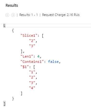
Figure 3-o: Result of the Scalar Query Using Array Manipulation Functions

Notice that Slice1 contains the values of the second and third values of the original array since we instructed the slice to occur on the item with index 1 (second item of the array because arrays use zero-based indexing) and we also instructed ARRAY_SLICE to fetch two items.

Also notice how Contains1 returns false, as the array doesn’t contain the value “5” and the result of ARRAY_CONCAT is assigned to an automatically generated property called $1, since no AS clause was provided for the last part of the scalar query.

Further documentation about these functions can be found here.

We’ve now seen what we can achieve with scalar queries. They provide a great way to manipulate results and create custom projections. Moving on, we’ll focus on querying real data that we’ll store in our collection.

Querying documents in a collection

We can really appreciate the value of DocumentDB’s SQL flavored query language when we have to use it to get data and project custom results from documents contained within a collection.

Once you include a FROM clause on a query, it is no longer a scalar query but instead a query that runs through all the documents within the current collection.

The name of the variable that goes after the FROM clause is merely an alias for the name of the current collection. Usually that alias is c, indicating the current collection, but it can be any other name.

Using the Data Explorer (Preview) blade, let’s add the following document to our current collection, which is available on Cosmos DB’s demo website. For a quick reminder on how to add a document, refer to the section “Adding a Document” from Chapter 2.

Code Listing 3-j: Sample Document

Now let’s run this next query.

Code Listing 3-k: Query for the Sample Document

After executing this query, we get the following result.

Code Listing 3-l: Custom Projection Query Results

There are a couple of things to notice. The first is that we were able to add a totally unrelated document to the one we had previously added, the one with data about Cristiano Ronaldo.

The document that we’ve just added has a structure, names, and values of properties that are totally unrelated to the original document we added to the current collection. This means we can add any type of document to a collection, with any kind of properties and values.

The second thing to notice is that in the query mentioned in Code Listing 3-k, we are using the alias Food to refer to the current collection, even though the collection might contain other documents that are unrelated to Food, such as the original one that contains data about Cristiano Ronaldo.

When we write a document query, it is recommended that we use an alias that represents the type of documents we are querying within the current collection. In this case, because we are querying about food, we have chosen to use the alias Food.

We could have chosen to use a generic alias like c, but by using the alias Food, we are simply making the query more readable and easier for us to understand in the future.

Also notice how the dotted notation is used to indicate the names of the properties that will be returned in the result and used for filtering (used inside the WHERE clause).

Using the dotted notation is required for a document query to work.

Querying using ORDER BY

Let’s move on and walk through the example queries listed on Cosmos DB’s demo website.

Go ahead and add this document to the current collection using the Data Explorer (Preview) blade within the Azure Portal.

Code Listing 3-m: Another Sample Document

Now let’s run this next query for the document that we’ve just added, using the Query tab.

Code Listing 3-n: Another Query for the Sample Document

Executing this query returns the following result.

Code Listing 3-o: Custom Projection Query Results

Because the servings property is an array with 3 items, by selecting food.servings[0].description, the query is retrieving the description subproperty of the first item within the servings array. This property is then projected as servingDescription.

It is also interesting to observe how DocumentDB has built-in support for ORDER BY and string range queries. Detailed information about using ORDER BY and how this relates to the indexing policy can be found here.

The TOP keyword

When there are many documents within a collection, it might be useful to limit the results to a certain number of documents. For instance, we might be interested in showing the first ten documents. This is where the TOP keyword comes in handy.

Take, for instance, the following example.

Code Listing 3-p: Query Using the TOP Keyword

In this query, we are instructing DocumentDB to return the top ten documents in the collection that match the filtering criteria of the query.

Since, at the moment, we only have one document that matches these criteria, when we execute this query, we get the same result as described in Code Listing 3‑l.

Figure 3-p: Result of the Query Using the TOP Keyword

However, that result could have been different if we had had more documents of that same type.

The IN and BETWEEN keywords

As mentioned on DocumentDB’s demo website, the IN keyword can be used to check whether a specified value matches any element in a given list. BETWEEN can be used to run queries against a range of values.

In order to understand this better, let’s add the following document to the current collection using the Data Explorer (Preview) blade.

Code Listing 3-q: Another Sample Document

Then add this one as well.

Code Listing 3-r: Another Sample Document

To see the IN and BETWEEN keywords in action, let’s look at the following query.

Code Listing 3-s: Query Using the IN and BETWEEN Keywords

Based on the two documents we just added to the current collection using Data Explorer, running this query returns the following result.

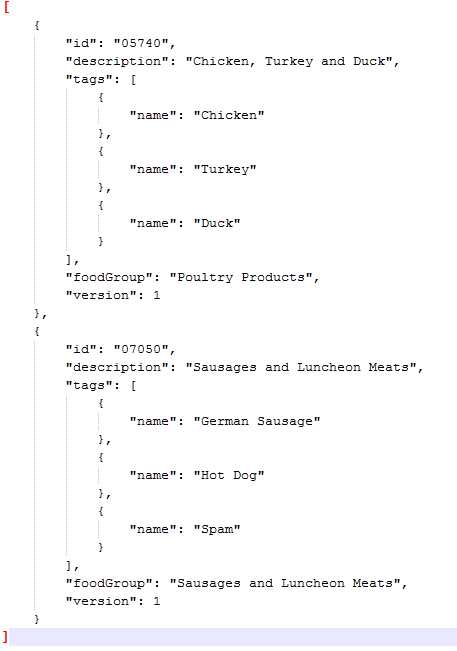
Figure 3-q: Result of the Query Using the IN and BETWEEN Keywords

The usage of the IN and BETWEEN keywords has allowed us to filter out the document mentioned in Code Listing 3-j, even though this document has the exact same properties as the documents mentioned in Code Listings 3-q and 3-r.

Using these keywords and narrowing the query down to any id property that is between a range of "05740" and "07050" inclusive have allowed us to specifically return the documents that matched the string criteria chosen for the foodGroup property.

If there had been other documents with a foodGroup of "Poultry Products" or "Sausages and Luncheon Meats," with id values between "05740" and "07050," these would have also been returned as part of the result.

We can quickly verify that this is true by adding the following sample document to the current collection using Data Explorer and afterwards running the same query again.

The following document is pretty much a clone of the document mentioned in Code Listing 3-r, except that we’ve modified its id to be "07049."

Code Listing 3-t: Another Sample Document

If we now run the query mentioned in Code Listing 3-s in the Query tab, we should also have as part of the result the document we’ve just added (mentioned in Code Listing 3-t). However, we still have filtered out the document mentioned in Code Listing 3-j. The result of the query would be as follows.

Code Listing 3-u: Result of the Query Using the IN and BETWEEN Keywords

Querying documents with projections

As mentioned, DocumentDB supports JSON projections within its queries. To see this in action, let’s add the following document to the current collection using Data Explorer.

Figure 3-r: Adding a New Document Using Document Explorer

Considering the following query, let’s see how we can project some custom properties as part of the result.

Code Listing 3-v: Query Using JSON Projections

Executing this query in the Query tab would return the following result.

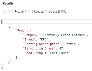
Figure 3-s: Result of the JSON Projections Query

The JSON object included in the SELECT clause of the query has allowed DocumentDB to project how the value of each property is returned in a different way, using alternative (more user-friendly) aliases.

JSON projections are a great way to customize results and make them more intuitive, user-friendly, and easier to read. They are especially convenient when writing queries that will be used to create reports.

Querying documents with JOIN

DocumentDB’s JOIN supports intradocument (within a document) joins but does not support interdocument (between different documents) joins.

Instead, the JOIN keyword is used to perform intradocument (nested) queries. In order to understand this better, let’s add the following document to the current collection using Data Explorer.

Code Listing 3-w: Another Sample Document

Having added this document to the current collection, let’s execute this next query that uses the JOIN keyword.

Code Listing 3-x: Query Using the JOIN Keyword

Running this query produces the following result.

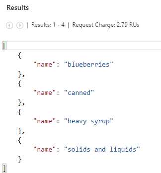
Figure 3-t: Result of the JOIN Query

If we take a moment to analyze this query, we can see that the JOIN focuses on the food.tags. In other words, the JOIN is narrowing down the scope of the query to the food.tags array and the rest of the document is ignored except for the food.id property, which is used in the WHERE clause of the query.

So, in essence, the JOIN allows the SELECT to focus on a specific section of the document.

As you can see, the JOIN in DocumentDB behaves in a totally different way than what you would expect from traditional T-SQL in a relational database.

This is likely the biggest difference between traditional SQL and DocumentDB databases.

Other interesting bits

DocumentDB has some other tricks up its sleeve. One of them is the ability to create an alias of an alias. This may sound redundant, but it’s a way to make queries shorter and write less.

Let’s look at an example query, which is a slight modification of the previous query that used the JOIN keyword.

Code Listing 3-y: Query Using the JOIN Keyword with an Alias

The trick is simply to re-alias the collection’s alias (food) to a shorter variable name, in this case f, using the AS keyword.

In this particular example, there’s no real added value to doing this. However, in a larger query with many more variables, re-aliasing is a great way to shorten the query by typing less.

In any case, it’s a nice trick. It’s good to know and use in particular situations, especially in long queries.

DocumentDB has another nice trick that allows us to retrieve only subsections of documents. The source can also be reduced to a smaller subset.

For instance, enumerating only a subtree in each document, the subroot could then become the source. Let’s explore an example.

Code Listing 3-z: Subroot Query

Any valid JSON value (not undefined) that can be found in the source will be considered for inclusion in the result of the query.

Executing this query will produce the following result.

Code Listing 3-aa: Execution of the Previous Query

Notice how the results returned correspond only to the servings subsections of the documents within the current collection and no other properties are even considered as the source of the information.

Documents within the collection that do not have a servings subsection are not even taken into account for the results.

Summary

Throughout this chapter, we’ve explored the various ways we can query DocumentDB directly from the Azure Portal using the built-in Query Explorer blade and a familiar SQL flavored syntax.

We’ve learned the basics of DocumentDB querying, explored scalar queries, and seen how to query documents independent of their structure, shape, and properties.

Even though the SQL flavored syntax looks very similar to what we are used to from the relational database world, we’ve also seen some differences and aspects that are unique to DocumentDB and give it a unique character.

DocumentDB’s querying capabilities are not only intuitive, but also rich and powerful. They provide a straightforward way of interacting with collections and are easy to implement and execute.

I highly recommend you keep exploring all the querying capabilities that DocumentDB has to offer. The official documentation website is a great resource to look at and read thoroughly.

So far it’s been an interesting journey and there’s more to explore. Up next, we’ll delve into the details of using DocumentDB from client code. This should also be fun and interesting to explore. Thanks for reading!