Your First Index

Solr’s Sample Data

At this point, you should have a running Solr instance and a good understanding of the tooling available to you in the Admin UI. Now, it’s time to start making Solr work for us.

Start by opening a command prompt and navigating to the exampledocs folder located within C:\solr-succinctly\succinctly\. If you shut down your Solr, start it again with java -jar start.jar. Make sure you do this in a different command prompt, however, as you'll need to type in the first one while Solr is running.

Within exampledocs, there are several CSV and XML files with sample data ready to be indexed and the distribution includes a simple command line tool for POSTing data to Solr, called post.jar. For instructions and examples on usage, use the following command:

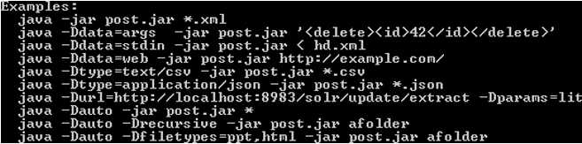
27. Help for post.jar

Before we start indexing any documents, let’s first confirm that we don't have any documents in the index. One way to do so is to navigate to the Admin UI, chose collection1 from the Core Selector, and click on Query. Then, at the bottom of the section, click Execute Query or click on any of the non-multiline text boxes, and push Enter.

All-in-all this constitutes quite a few steps—there is, however, a quicker way. Navigate directly to Solr via its RESTful interface, querying for all documents. This will not use the Admin UI; it will just run the query. The URL looks like this:

As you can see in the results, we have zero documents in our index.

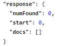
28. No documents in the index

Time to upload the sample data. From exampledocs in your command prompt, type:

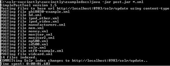
29. POST example files

All the XML files supplied have been posted directly into my index and have been committed; this has all been done automatically by the POST tool. It's also worth noting that a simple mistake that many people make is they post data to the index, but forget to commit. Data is only ever available for searching if you remember to execute the commit; however, since the post tool does this for you automatically, it's a mistake you often won't make.

Post.jar is only one way of indexing documents. Another mechanism is the data import handler, which allows connections to databases and imports data in either full or incremental crawls. You can also add XML, JSON, CSV, or other types of files via the Documents section in the Admin UI. Additionally, you can use a client library, like SolrNet or SolrJ, and there are multiple content-processing tools that post documents to the Solr index. One that I see being used all the time is Search Technology’s ASPIRE, which has a PostToSolr functionality.

Switch back to your browser and run the default query again. You should now see 32 documents in your index. The following figure shows the output you should now get, allowing you to become familiar with Solr responses.

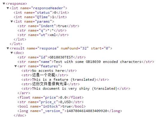
30. Example documents indexed

At this point, you’ve run a couple of queries, which amounts to asking your search engine to perform a basic query. You did this in two ways: first by using the Query section in the Admin UI, and second by using Solr’s RESTful interface.

31. Solr query

Simple Anatomy of a Query and a Response Query

If you select a core, click Query, and press Enter, you will be able to see a query and a response. In this section, we'll start to really understand what is actually happening by using the sample data we just uploaded into collection1.

Tip: If your browser supports XML formatting (like Google Chrome does), you can make a quick change for easier readability. Please open the response in your browser, look for the wt=json parameter in the URL, and change to wt=xml. The wt is the response writer, which tells Solr how to format the response. Try it.

As we've seen so far, Solr uses a fairly standard RESTful interface, which allows you to easily see the URL used to make a query; like any standard URL, it’s made up of the host name, the port number, and the application name.

The request handler for queries (in this case we're using select) is the default request handler, and is the Solr equivalent of “Hello World.” The default query of exampledocs is made up of the following URL parameters:

Like with any technology, the best way to learn and understand is to play with it; imagine Solr's default install as your big data and enterprise search training wheels. Open the Admin UI, change the parameters, and see how your results are modified and what differences your changes make to the search. Once you've tried a few queries and gotten a feel for how they work, you’re ready to move on.

Response

When you run a query, the response you get will contain two full sections:

• ResponseHeader
• Response

You can see an example in the following figure:

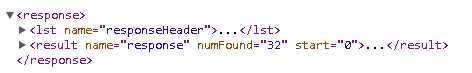
32. Solr response

The ResponseHeader contains information about the response itself. The status tells you the outcome; 0 stands for OK. If you query for a nonexistent request handler, you would get a 404 response code as the HTTP response.

The ResponseHeader also includes QTime, which is the query execution time and echoing of the parameters.

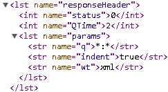
33. Response header

The response section includes the results of those documents that matched your query in doc subsections or nodes. It includes a numFound that indicates how many documents matched your query, and start, which is used for paging.

Other Response Sections

• highlighting: Allows fragments of documents that match the user's query to be displayed in the response.
• facet_counts: Shows the facets that have been constructed for the result list, including the facet fields and facet values (with counts) to populate each field.
• spellcheck: Will include suggestions for possible misspellings in the user's query.
• debug: Intended for development and debugging. Only included if specified as part of the query. Among its subsections, it includes explain to understand how each document scored according to the in-relevancy ranking algorithm, and timing to understand how long each component took for processing. In parsedquery, it displays how the query string is submitted to the query parser.

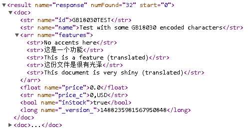
34. A Solr document

Docs and Modeling Your Data

You are probably wondering at this point how we model our data within Solr. That’s where one of the main configuration files comes into play—you model your data and specify to Solr how to handle it in the Schema.xml file. The following figure shows an example.

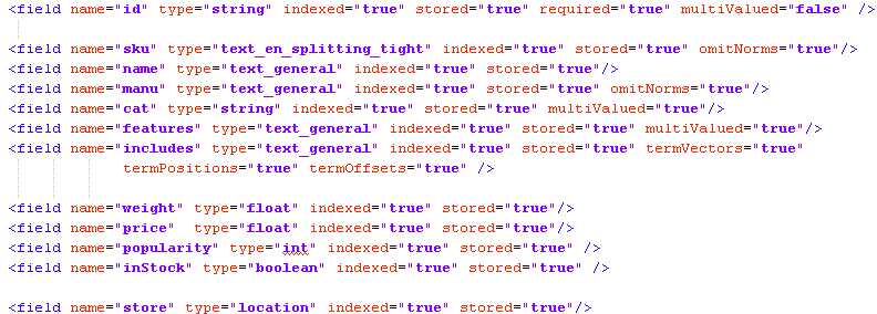
35. Example docs schema

Each document has a set of fields, and each field can be of a different type. In this specific sample case for the documents we just uploaded, we can see that we have id, sku, name, manu, cat, features, includes, weight, price, popularity, inStock, and store.

The schema also includes a series of common metadata fields, named specifically to match up with Solr Cell metadata.

Note: Solr Cell is a functionality that allows sending rich documents such as Word or PDF documents directly to Solr for parsing, extraction, and indexing for search. We will not be covering SolrCell in this book.

To use an analogy: if you are familiar with databases, then a doc would correspond to a row. The name would be the column name, and type is exactly the same thing—it indicates what type of information will be stored in this specific field. Required indicates if it is mandatory, just like specifying NOT NULL in the structured query language.

The ID in this specific case is just like the primary key, the unique id for the document. It is not absolutely required, but highly recommended. You specify which field you want to be the primary key in the schema in <uniquekey>.

36. Unique key ID

And now let’s get to some specifics:

• Indexed=“true|false” is used to specify that this specific field is searchable. It has to be added to the index to be searchable.
• Stored=“true|false” can be hard to swallow at first. If you specify that a field is not stored, then whenever you run a query, the original value of that field is not returned. There is, however, one point that is very important. You can set a field to stored=“false” and indexed=“true”, meaning that you index the data, but the data itself for that field is not saved in Solr, so you can’t extract it as part of the results.

Note: While this might seem counter-intuitive, there's actually a pretty simple reason for it. Let’s imagine you have some very large fields and you don’t care about retrieving the full text; e.g. finding which documents contain the specific terms searched. This gives you a very fast search solution with a very low memory footprint, allowing the client to retrieve the larger amount of data at his own discretion.

• Multivalued=“true|false” indicates whether you want to hold multiple fields within the same field. For example, if a book has multiple authors, all of them would be stored in one field.

Solr supports many different data types, which are included in the Solr runtime packages. If you want to get very technical, they are located in the org.apache.solr.schema package.

Here is the list according to Solr’s wiki:

It is worth mentioning that there is something called Schemaless mode, which pretty much allows for you to add data without the need to model it, as well as dynamic fields. We will not be covering them in this book.

Playing Around with Solr

With our first Solr “Hello World” query, we simply looked for *:*, meaning all values for all fields, which returned all 32 documents. Let’s raise the stakes a notch and play around with a few queries, changing different parameters as we go. We won’t get too complicated; we’ll just show a few examples to help you understand some of the basic functionalities of Solr.

A “Real” Query with Facets

In this example, we will run a specific query of *:* and ask for facets to be included.

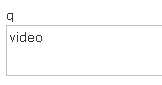
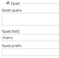
Using the cores dropdown menu in the Admin UI, select the collection1 core, type in video in the q field, check facet, and select xml as the response writer (wt). Type in manu as the facet field and execute the query using the Execute Query button.

It should look like this:

37. Running a query

Two things should definitively stand out from the response. First, you will see only relevant results; in this case, three documents matched instead of 32.

38. Three documents found

More importantly, you can now see facets for manu. We will get into more details later about facets, but for now please take a look at the list within facet_fields called manu, which holds the list of all manufacturers, sorted from highest occurrence to lowest. It includes the names and a count. Facets are also called navigators, and they allow drill down on specific result sets. In this example, given that the list is very long, I have included an ellipsis (…) to indicate that there are many more results, mainly with 0 values; you can see this reflected in the figure below.

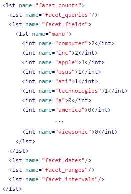
39. Facets

Fields

At the present moment we are returning all fields, which may or may not make sense, depending on your specific needs. If you need to provide all fields back to the application, then there is no need to use fl (fields) input. If you want smaller responses to help with performance, especially when using large documents, just include the list of fields that you want returned in fl. Simply type them in separated by a blank space or comma. This also helps with readability while querying for testing.

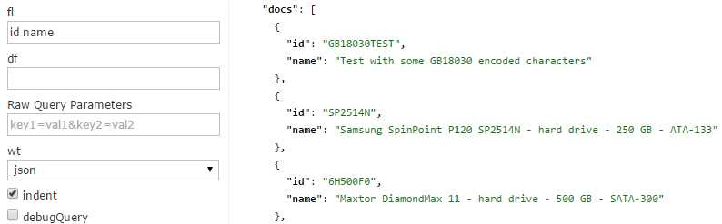
40. Returning specific fields

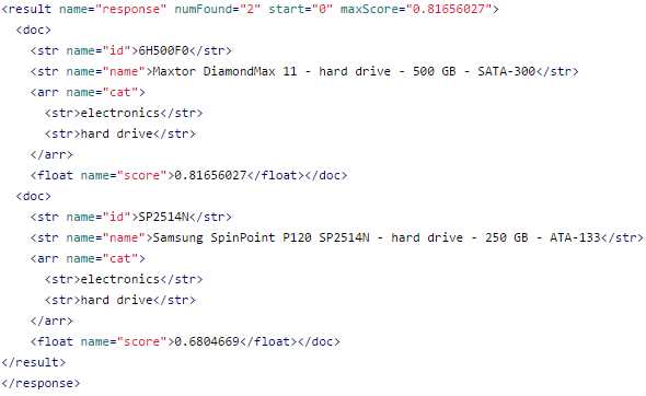
A very neat and useful trick is to include score as a field, which will tell you the score (or how relevant a document is) from the result set. Try adding a query to the previous search; I will add q=drive, include the score field, and execute and analyze the results, as you can see in the fl field in the following figure.

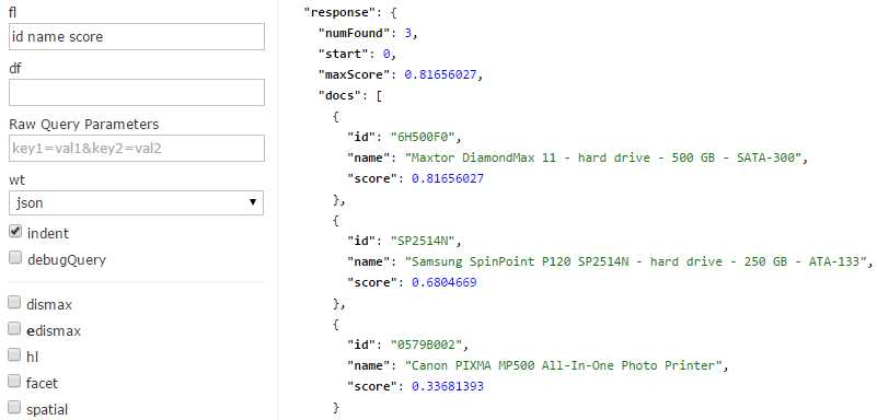
41. Include Score as a Field

Results are ranked from highest to lowest score, or most relevant to least relevant. That is, of course, if no other sorting is applied.

Sorting

To take advantage of the ability to select which fields to display, let’s try sort. Sorting to a query is a very simple process—simply type in the field you want to sort on, and then either asc (ascending) or desc (descending), as the next figures demonstrate.

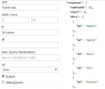
42. Sorting ascending

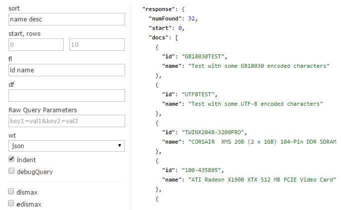
43. Sorting descending

You can also sort on more than one field at a time. To do this, simply specify the field name, the sort direction, and then separate the groups with a comma. For example: name desc, id asc.

Paging: Start and Rows

You can add paging to your applications using Start and Rows. Start is the offset of the first record that you are returning. For example, if you run a query, 10 results are returned by default. You know that you want the second page, so you run the same query, but with start=11 and rows=10, thus producing the second page also containing 10 results.[1]

Learning the Difference between Queries (q) and Filter Queries (fq)

I have already mentioned how q calculates results based on relevancy, and fq is only used to drill down. I also mentioned that fq is very efficient in terms of performance; the reason for this is that filter queries cache results and only stores ids, making access very fast. Now that we’ve learned how to get a score for our results, we can prove that this is indeed the case.

The steps to do this are very simple:

10. Open two windows, and in each one, navigate in the Admin UI to the query section of collection1. You will be running in both windows. Write down drive and include the following four fields in the fl section: id name cat score. For readability, if your browser supports nice XML formatting, please change wt to xml.

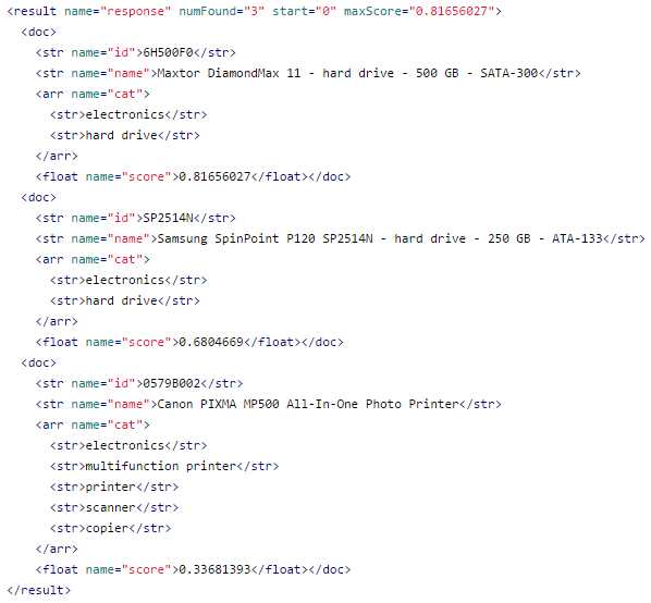
44. Query for drive

11. When you execute the query you will get three results, two of which have a category of “hard drive.”

We just ran a query using the q field. Let’s now run a new query using fq instead. The intention is to prove how q and fq affect queries in a different way. The bottom line is that q affects ranking, while fq does not. It is extremely important to understand this difference, as using them incorrectly will bring results that are not as relevant as they should be.

Query

Please reload the Admin UI in both windows so that we can start from clean query pages.

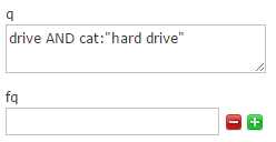
In one of the windows, add in the q input box the following query: drive AND cat:“hard drive”. Be careful with capitalization, and remember to include the following four fields in the fl section: id name cat score. Your query should look like the following.

45. No filter query

Your result should look like this:

46. No filter query response

Filter Query

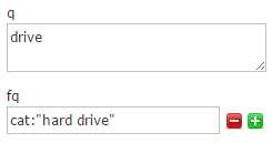
In the other window, set q=drive and add cat:“hard drive” within fq. As before, include the four fields in the fl section: id name cat score. Your query should match the following:

47. Query and filter query

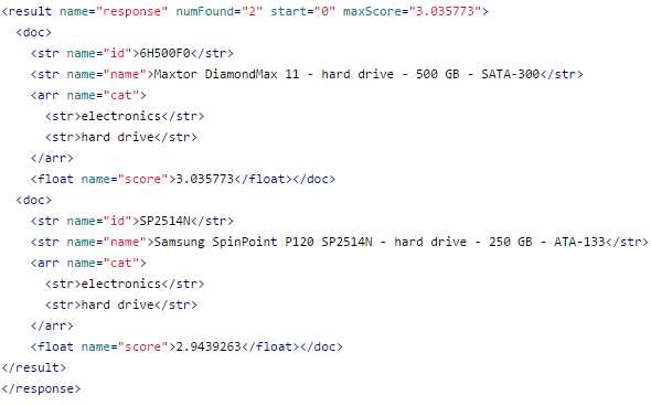
You will get the following result:

48. Query and filter query response

When you look at the response results, using 'fq' doesn't affect the score. The first run took the longest, and the second was quicker. The third run using 'fq' has not changed at all, showing that Solr has just returned the results already cached from the previous queries.

Summary

In this chapter, you’ve learned how to load Solr’s sample documents and how to run a few simple queries. We’ve discussed the anatomy of a simple query and response, and finally, proved the difference between q and fq in terms of ranking. In the next chapter, we'll continue by learning how to create a schema for our own documents.